Visualizing sedflux Output

There are two main sedflux output files: a property file, and a measuring station file. Both can be visualized with Matlab mfiles located in the sedflux-mfiles GitHub repository.

Sedflux Property File

Sedflux property files are those generated by the Data Dump processes specified in the process file. For sedflux2D these are stratigraphic cross-sections that record properties such as grain size, age, and bulk density. For sedflux3D, these files describe data cubes. These files can be plotted in Matlab with the sedflux plot_property function.

sedflux2D: plot_property

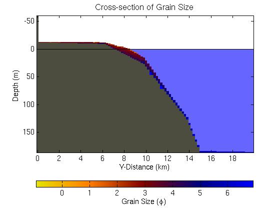
For our first example, we consided a property file of average grain size that was generated by sedflux run in 2D-mode. For the simulation called, sedflux_2D_simulation, we can use the following to look at some output,

>> plot_property ('sedflux_2D_Simulation0001.grain');

If all goes well, MATLAB should generate an image of the average grain size over the profile.

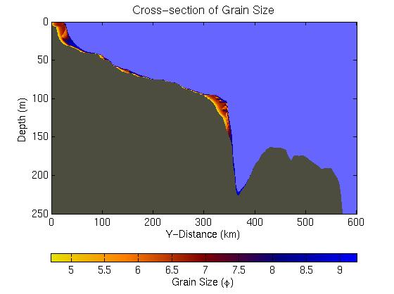
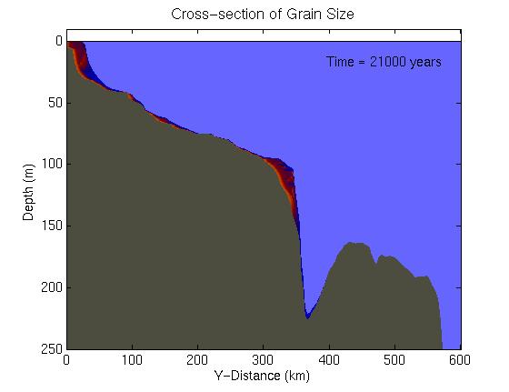
Following the name of the file, the user can specify a series of parameter/value pairs that control how the image is displayed. For instance, the following parameter/value pairs print the time (in years), scale the data between 2 and 10 (phe units), and remove the colorbar.

>> plot_property ('sedflux_2D_Simulation0001.grain' , 'time' , 21000 , 'clim' , [2 10] , 'colorbar' , false);

Other parameters are func, and mask. Use func to specify a function handle that will operate on the property data. The function should take a matrix as its only input parameter. Continuing with the previous example, we can plot grain size in millimeters rather than phe units using the func parameter.

>> plot_property ('sedflux_2D_Simulation0001.grain' , 'func' , @(f)(2.^(-f)));

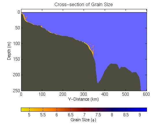
A data mask is a matrix of logical values that is the same size as the data to be plotted. To create a mask, one usually reads in the data and then creates the mask based on those data values. This requires the MATLAB function read_property (explained later). In the following example, we wish to only plot those data between 2 and 6 phe units.

>> [f,h] = read_property ('sedflux_2D_Simulation0001.grain');
>> plot_property ('sedflux_2D_Simulation0001.grain' , 'mask' , f>2 & f<6);

sedflux3D: plot_property

The following MATLAB command plots a slice of sedflux 3D cube. In this example we plot a slice of grain size along the plane at x=3.2km. One can also specify a slice of constant y or z (use ‘yslice’ or ‘zslice’, respectively).

>> plot_property ('sedflux_3D_Simulation0001.grain' , 'xslice' , 3.2);